A ten-minute tour of NCToolkit's core abilities, using a historical global sea-surface temperature dataset served over a thredds server.
We'll use monthly average sea-surface temperature for 1991–2020 from NOAA's COBE-SST 2 dataset, read directly from a thredds server — no download needed.
The preferred way to import the package is as nc:
import nctoolkit as nc
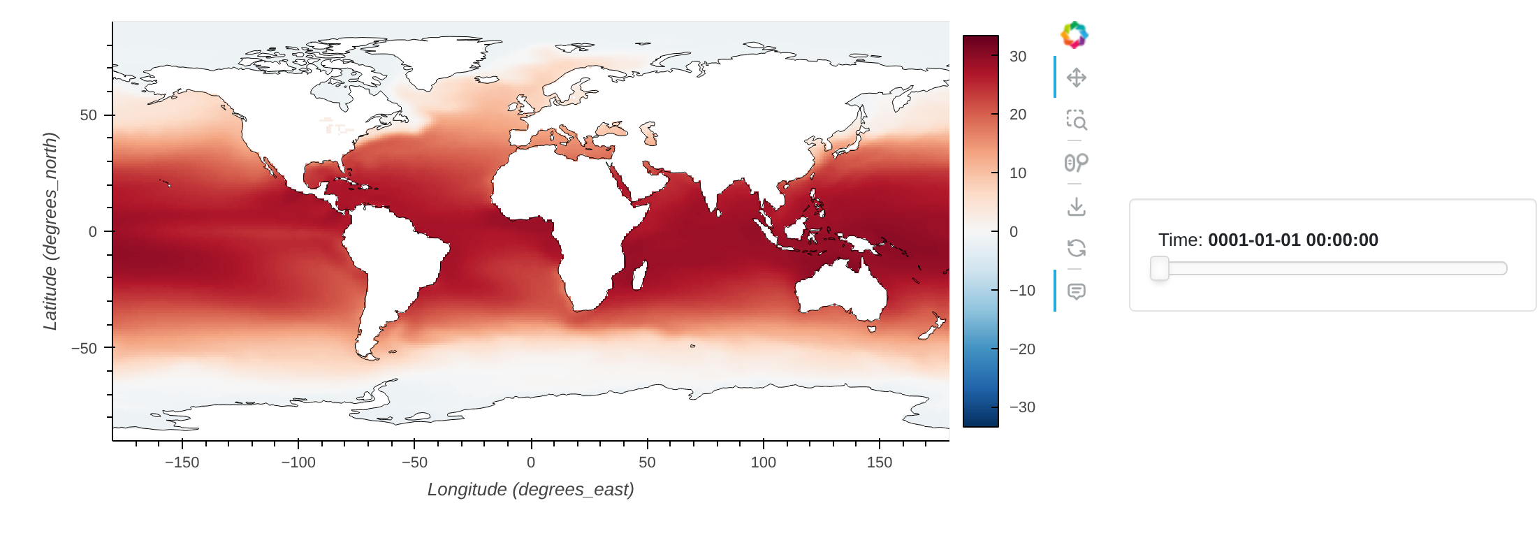
NCToolkit offers automatic plotting for almost any netCDF file. Calculating and plotting mean historical sea surface temperature is as simple as:
ds = nc.open_thredds("https://psl.noaa.gov/thredds/dodsC/Datasets/COBE2/sst.mon.ltm.1991-2020.nc")
ds.plot()
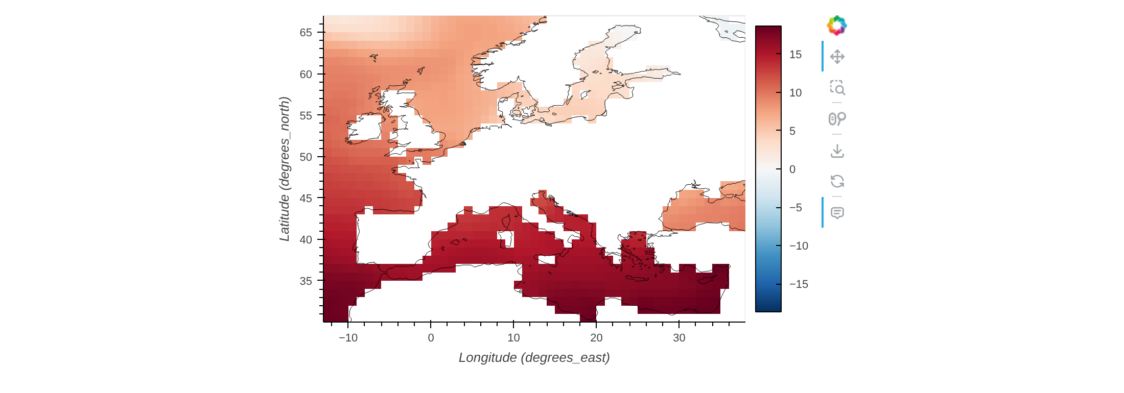
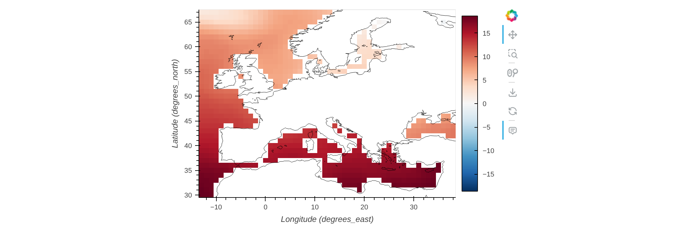
To look at a particular region, use subset. Here we select January and crop to a European box:
ds = nc.open_thredds("https://psl.noaa.gov/thredds/dodsC/Datasets/COBE2/sst.mon.ltm.1991-2020.nc")
ds.subset(month=1, lon=[-13, 38], lat=[30, 67])
ds.plot()
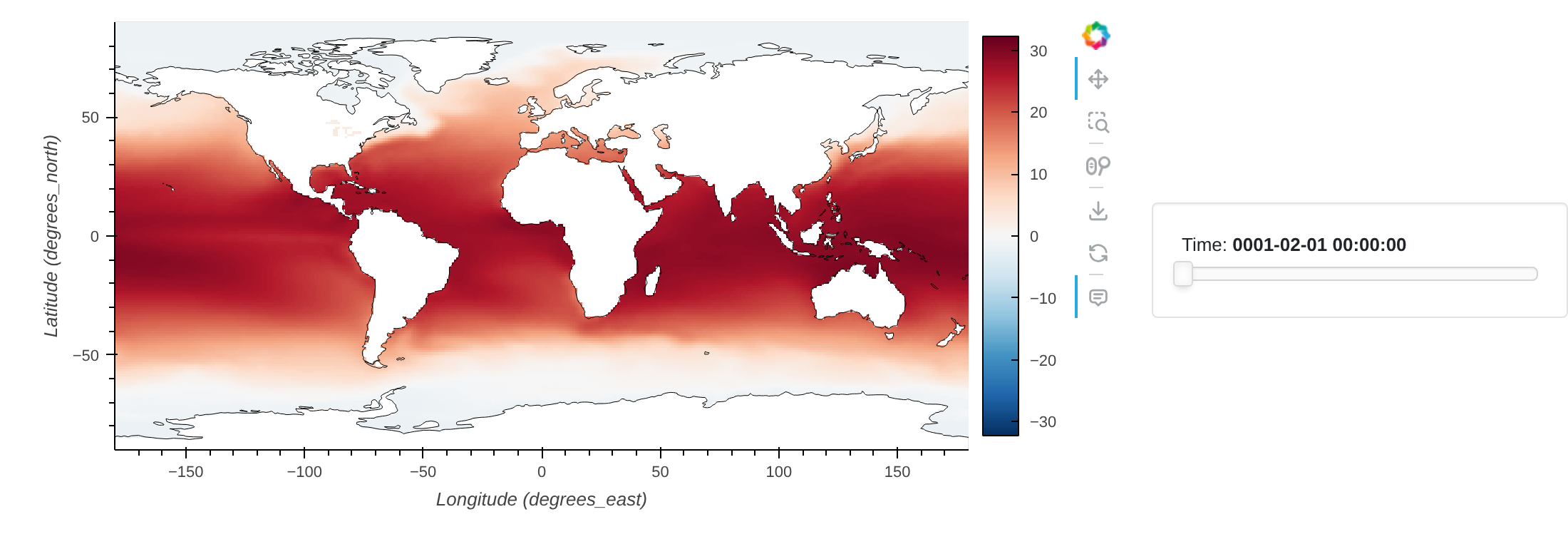
A suite of methods prefixed with t calculate temporal statistics. A seasonal average:
ds = nc.open_thredds("https://psl.noaa.gov/thredds/dodsC/Datasets/COBE2/sst.mon.ltm.1991-2020.nc")
ds.tmean("season")
ds.plot()
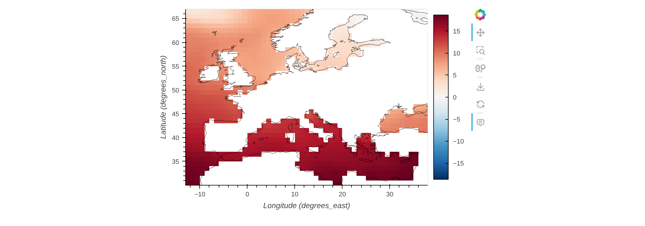
And spatial averages are just as simple:
ds = nc.open_thredds("https://psl.noaa.gov/thredds/dodsC/Datasets/COBE2/sst.mon.ltm.1991-2020.nc")
ds.subset(variables="sst")
ds.subset(lon=[-13, 38], lat=[30, 67])
ds.spatial_mean()
ds.plot()
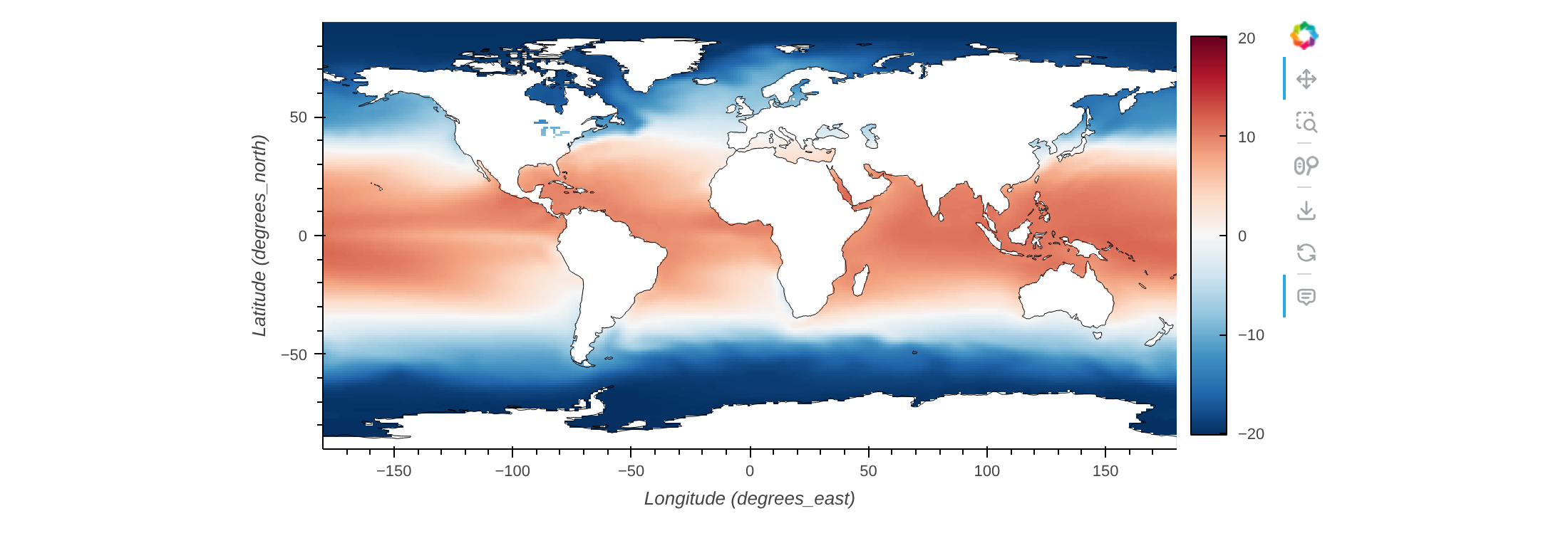
The assign method works like pandas' assign. Here's how much warmer each part of the ocean is than the global mean:
ds = nc.open_thredds("https://psl.noaa.gov/thredds/dodsC/Datasets/COBE2/sst.mon.ltm.1991-2020.nc")
ds.tmean()
ds.assign(delta=lambda x: x.sst - spatial_mean(x.sst), drop=True)
ds.plot()
Built-in methods handle horizontal and vertical interpolation. to_latlon regrids to a regular lon/lat grid — just give it the extent, resolution and method:
ds = nc.open_thredds("https://psl.noaa.gov/thredds/dodsC/Datasets/COBE2/sst.mon.ltm.1991-2020.nc")
ds.to_latlon(lon=[-13, 38], lat=[30, 67], res=1, method="bil")
ds.plot()
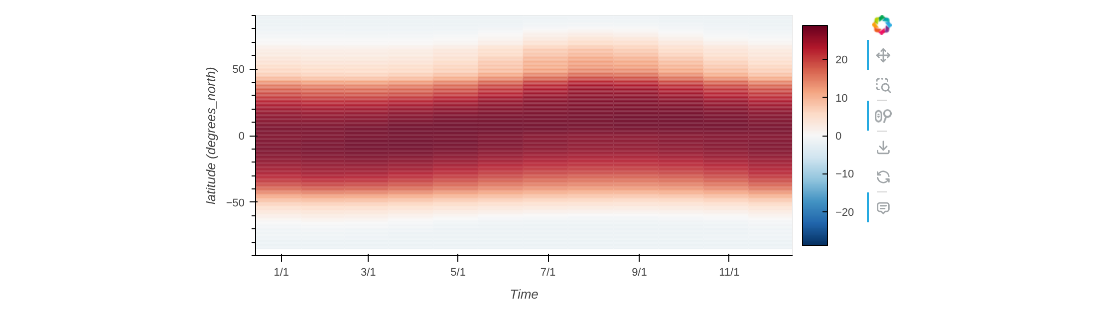
ds = nc.open_thredds("https://psl.noaa.gov/thredds/dodsC/Datasets/COBE2/sst.mon.ltm.1991-2020.nc")
ds.zonal_mean()
ds.plot()
That's the shape of it: open a dataset, chain a few methods, and plot or export the result. From here: