Sea surface sea temperature validation using gridded observations from COBE2#
Matchup procedure: The model and observations were matched up as follows. First, the model dataset was cropped by a small amount to make sure cells close to the boundary were removed. The model was then regridded to the observational grid using bilinear remmaping. Only grid cells with model and observational data were maintained. The following model output was used to compare with the observational values: tos.
Baseline climatologies of sea surface sea temperature
Climatologies of model and observational sea surface sea temperature are shown in the figures below. The model climatology is calculated using the year 2014.
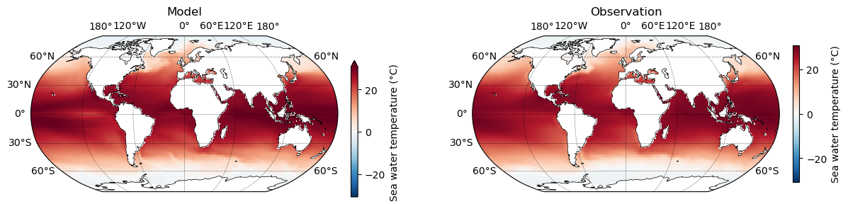
Figure 1: Annual average surface sea temperature from the model (2014) and observations. Data is limited to the 2nd and 98th percentile of the combined model and observational data. Arrows indicate that values can exceed the colorbar limits.
Assessing model bias for surface sea temperature
Figure 2 shows the average bias of surface sea temperature simulated by the model. A positive bias indicates that the model overestimates the observation, while a negative bias indicates that the model overpredicts the observation.
The spatial average bias of surface sea temperature is 0.66 degC. Overall, the model overestimates the observations in 74.5% of the model domain.
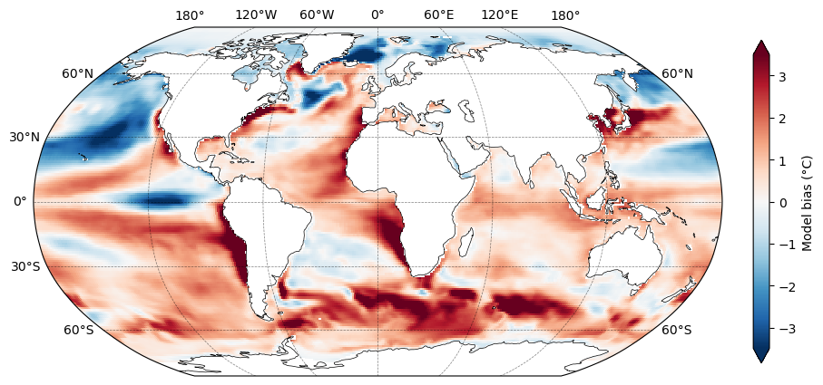
Figure 2: Bias of surface sea temperature from the model. A positive bias indicates that the model overestimates the observation. For clarity, the colorbar is limited to the 2nd and 98th percentile of the data.
Can the model reproduce seasonality of sea surface sea water temperature?
The ability of the model to reproduce seasonality of sea surface sea temperature was assessed by comparing the modelled and observed seasonal cycle of sea temperature. First, we derive a monthly climatology for the model data. Then, we calculate the Pearson correlation coefficient between the modelled and observed sea temperature at each grid cell.
Note: we are only assessing the ability of the model to reproduce the ability of the model to reproduce seasonal changes, not long-term trends.
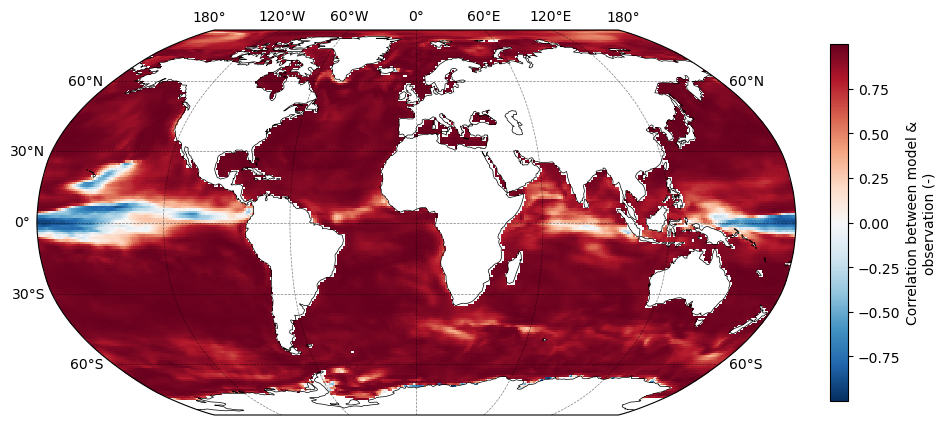
Figure 3: Seasonal temporal correlation between model and observations for surface sea temperature. This is the Pearson correlation coefficient between climatological monthly mean values in the model and observations.
The seasonal cycles of simulated and observed sea temperature are compared in Figure 4 below. This figure shows the model and observation average in each month of the year, and the differences between the two each month
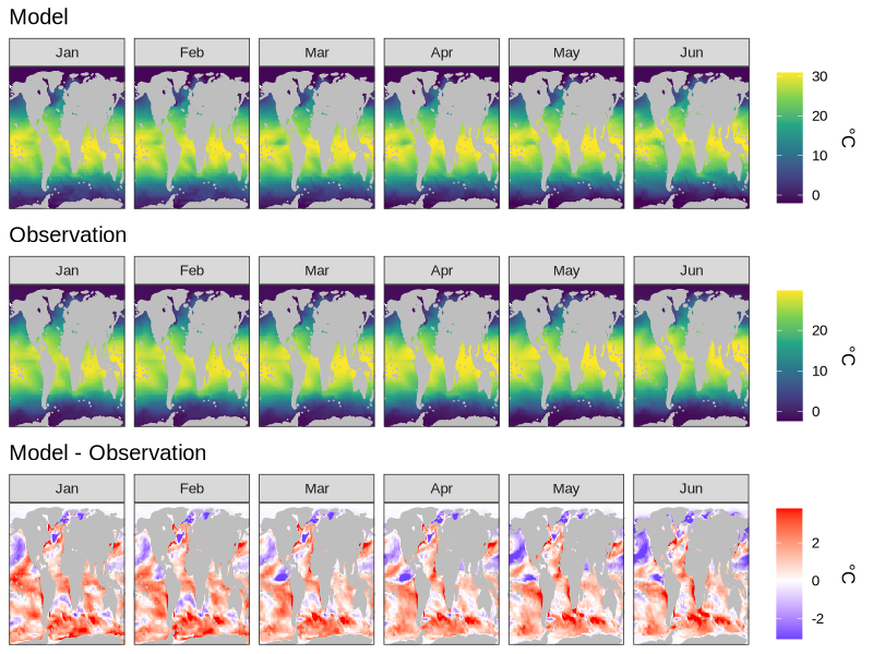
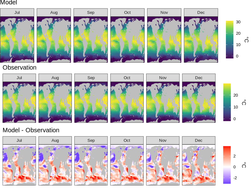
Figure 4: Monthly mean surface sea temperature for the model, observation and the difference between model and observations. For clarity, the maximum values are capped to the 98th percentiles.
Regional assessment of model performance for sea surface sea water temperature
We assessed the regional performance of the model by comparing the model with observations in a number of regions. The regions considered are mapped below.
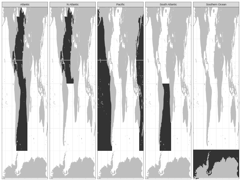
Figure 5: Regions used for validation of sea surface sea water temperature.
Time series were constructed comparing the monthly mean of the spatial average sea surface sea temperature in each region. The spatial average was calculated using the mean of all grid cells within each region, accounting for grid cell area.
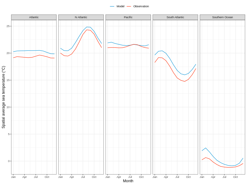
Figure 6: Seasonal cycle of sea surface sea water temperature for model and observations for each region. The spatial average is taken over the region.
The table below shows the average bias of sea surface sea temperature in each region. The bias is calculated as the modelled value minus the observed value. A positive bias indicates that the model overestimates the observed value, while a negative bias indicates that the model underestimates the observed value.
| Region | Spatial correlation | Temporal correlation | Bias | RMSD |
|---|---|---|---|---|
| Atlantic | 0.99 | 0.93 | 1.02 | 1.87 |
| North Atlantic | 0.99 | 0.93 | 0.82 | 1.70 |
| Pacific | 0.98 | 0.76 | 0.42 | 1.79 |
| South Atlantic | 0.99 | 0.94 | 1.23 | 2.02 |
| Southern Ocean | 0.92 | 0.88 | 0.85 | 1.30 |
Table 1: Summary of performance of the model sea surface sea water temperature in each region. The bias (°C) column represents the spatial average of the annual mean modelled value minus the observed value. The temporal correlation column represents the spatial mean of the temporal correlation between the model and observations per grid cell. The spatial correlation column represents the spatial correlation between the model and observations.
Can the model reproduce spatial patterns of sea surface sea water temperature?
The ability of the model to reproduce spatial patterns of sea surface sea temperature was assessed by comparing the modelled and observed sea temperature at each grid cell. We calculated the Pearson correlation coefficient between the modelled and observed sea temperature at each grid cell.
This was carried out monthly and using the annual mean in each grid cell
| Time period | r |
|---|---|
| Annual mean | 0.99 |
| Jan | 0.99 |
| Feb | 0.99 |
| Mar | 0.99 |
| Apr | 0.99 |
| May | 0.99 |
| Jun | 0.99 |
| Jul | 0.98 |
| Aug | 0.98 |
| Sep | 0.98 |
| Oct | 0.99 |
| Nov | 0.99 |
| Dec | 0.99 |
Table 2: Pearson correlation coefficient between modelled and observed sea surface sea water temperature at each grid cell. The correlation was calculated monthly and using the annual mean in each grid cell.
Data Sources for validation of sea temperature
COBE-SST 2 and Sea Ice data provided by the NOAA PSL, Boulder, Colorado, USA, from their website at https://psl.noaa.gov/data/gridded/data.cobe2.html.