A common challenge when working with netCDF data is matching it up with point observations — often sparse in space and time, and at varying depths.
Matching gridded data to point observations is handled by match_points. We'll illustrate this with ocean nitrate from NOAA's World Ocean Atlas, cropped to part of the North Atlantic:
import nctoolkit as nc
ds = nc.open_thredds("https://data.nodc.noaa.gov/thredds/dodsC/ncei/woa/nitrate/all/1.00/woa18_all_n01_01.nc", checks=False)
ds.crop(lon=[-40, 20], lat=[40, 70], nco=True)
ds.subset(variables="n_an")
ds.plot()
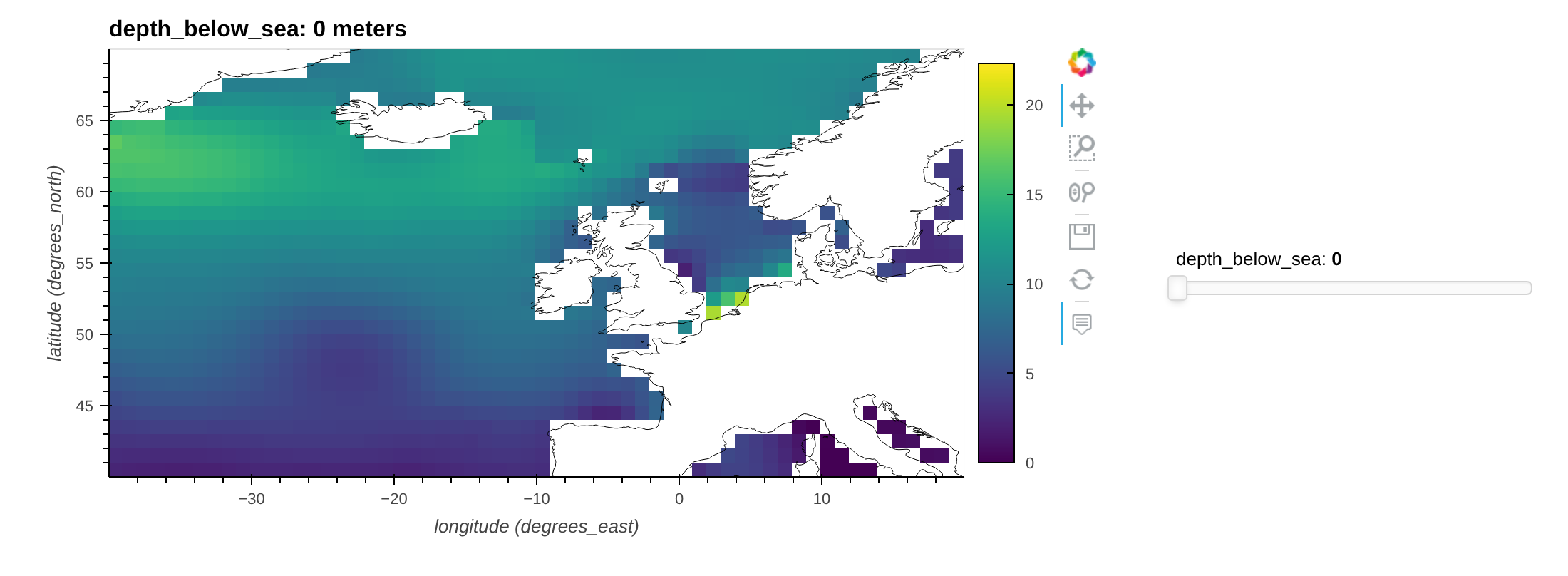
That covers nitrate from the sea surface to the sea floor. The dataframe of points must use column names from lon, lat, depth, year, month or day. Given a dataframe of four coordinates and depths:
import pandas as pd
df = pd.DataFrame({"lon":[-10, -12, -14, -16], "lat":[45, 50, 53, 55], "depth":[4, 2, 30, 40]})
df
| lon | lat | depth | |
|---|---|---|---|
| 0 | -10 | 45 | 4 |
| 1 | -12 | 50 | 2 |
| 2 | -14 | 53 | 30 |
| 3 | -16 | 55 | 40 |
Note: the dataframe columns must be named one of lon, lat, depth, year, month or day. To match our dataset to this dataframe:
ds.match_points(df)
| lon | lat | depth | n_an | day | month | year | |
|---|---|---|---|---|---|---|---|
| 0 | -10 | 45 | 4 | 5.661312 | 16 | 1 | 1958 |
| 1 | -12 | 50 | 2 | 8.932839 | 16 | 1 | 1958 |
| 2 | -14 | 53 | 30 | 8.672163 | 16 | 1 | 1958 |
| 3 | -16 | 55 | 40 | 6.973096 | 16 | 1 | 1958 |
match_points returns a pandas dataframe with the matched-up values added. Watch for messages confirming assumptions NCToolkit made while matching — usually safe to ignore, except around depths, which are derived from the dataset unless you provide them explicitly. For the example above, NCToolkit reports:
Depths assumed to be [0.0, 5.0, 10.0, …, 800.0]
All variables will be used
Points will be matched for all time steps
Data is first regridded horizontally using bilinear interpolation to the given lon/lat pairs. If depths are provided, the result is then interpolated vertically using 1D interpolation (via scipy).
The same method handles matchups over time — illustrated here with daily air temperature from the CMIP6 model GFDL-CM4. Given a dataframe with lon, lat, year, month and day columns for two points at different times:
df = pd.DataFrame({"lon": [50, 60], "lat": [50, 45], "year":[1850, 1852], "month":[1, 3], "day":[2, 3]})
df
| lon | lat | year | month | day | |
|---|---|---|---|---|---|
| 0 | 50 | 50 | 1850 | 1 | 2 |
| 1 | 60 | 45 | 1852 | 3 | 3 |
This only contains two data points, but for different times. Match up as before:
ds = nc.open_data("tas_day_GFDL-CM4_historical_r1i1p1f1_gr1_18500101-18691231.nc", checks=False)
df_match = ds.match_points(df)
df_match
| lon | lat | tas | year | month | day | |
|---|---|---|---|---|---|---|
| 0 | 50.0 | 50.0 | 252.836945 | 1850 | 1 | 2 |
| 1 | 60.0 | 45.0 | 271.053040 | 1852 | 3 | 3 |
As expected, a dataframe with surface air temperature for the locations and times specified. match_points works like pandas' merge: specify only year and month, omitting day, and every day for those years and months is returned:
df_match = ds.match_points(df.drop(columns="day"))
df_match
| lon | lat | tas | year | month | day | |
|---|---|---|---|---|---|---|
| 0 | 50.0 | 50.0 | 254.234680 | 1850 | 1 | 1 |
| 1 | 50.0 | 50.0 | 252.836945 | 1850 | 1 | 2 |
| 2 | 50.0 | 50.0 | 252.467865 | 1850 | 1 | 3 |
| 3 | 50.0 | 50.0 | 253.731049 | 1850 | 1 | 4 |
| 4 | 50.0 | 50.0 | 245.843506 | 1850 | 1 | 5 |
| … | … | … | … | … | … | … |
| 57 | 60.0 | 45.0 | 276.231720 | 1852 | 3 | 27 |
| 58 | 60.0 | 45.0 | 277.647888 | 1852 | 3 | 28 |
| 59 | 60.0 | 45.0 | 275.756226 | 1852 | 3 | 29 |
| 60 | 60.0 | 45.0 | 274.968018 | 1852 | 3 | 30 |
| 61 | 60.0 | 45.0 | 277.621979 | 1852 | 3 | 31 |
62 rows × 6 columns
We now have every day for the given times.
A handful of arguments refine the matchup process: variables, tmean, top and nan.
variablesRestrict the matchup to a subset of variables, e.g. ds.match_points(df, variables="tas").
tmeanApply ds.tmean() with the temporal grouping implied by the dataframe columns before matching — useful when point data is coarser than the dataset (e.g. monthly points, daily data). This is equivalent to running ds.tmean(["year", "month"]) beforehand.
topWhen the dataset has multiple vertical levels but you only want the top one.
nanValues in the dataset that should be treated as missing.
Using tmean with monthly points against the daily dataset above:
df = pd.DataFrame({"lon": [50, 60], "lat": [50, 45], "year":[1850, 1852], "month":[1, 3]})
df_match = ds.match_points(df, tmean=True)
df_match
| lon | lat | tas | year | month | day | |
|---|---|---|---|---|---|---|
| 0 | 50.0 | 50.0 | 256.112976 | 1850 | 1 | 16 |
| 1 | 60.0 | 45.0 | 271.545959 | 1852 | 3 | 16 |